How To Group Rows (comma list of values)

Hello and welcome to our post on grouping rows in Excel. We will walk through the process of combining the values in multiple rows into a single cell (comma-separated list of values). The example we’ll use to demonstrate the steps is to combine multiple email addresses for each contact into a single cell. But, this technique works on any set of data values, not just email addresses.

Video

Step-by-step Walkthrough

This discussion revolves around two key Excel features: Tables and Power Query. Tables help organize and store data in a structured way, while Power Query aids in data manipulation tasks. We’ll show how these Excel features can assist in grouping rows together. Let’s dive right in!

Exercise 1: Transforming data range into a Table

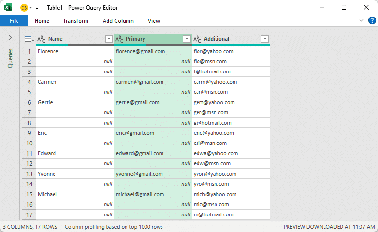
The first thing we’ll want to do is convert our ordinary data range into a Table. In this illustration, we have several contacts. Each contact has a first name, primary email address, and then multiple additional email addresses. Our sample data looks a bit like this:

Our goal is to collapse the rows, so that each contact has a single row. The single row should contain these columns: first name, primary email, and additional emails (which should contain a comma-separated list of additional email addresses).

To convert this ordinary data range into a Table, select any cell within the range and click on Insert >Table. Assuming the data has header rows (ie, column labels), be sure to check the ‘Table has Headers’ checkbox in the resulting Create Table dialog. The data is now stored in a Table:

Storing data in a Table helps future updates, since it will auto-expand as new data is added.

With that step complete, it is time to use Excel’s Power Query feature to transform the data.

Exercise 2: Employing Power Query

With the Table in place, it’s now time to use Power Query. Select any cell in the Table and use the Data > From Table/Range command to open the Power Query editor:

The Primary column includes empty or null values. We need to fill those with emails addresses to prepare for our next step of grouping. So, we select the Primary column and use the Transform > Fill > Down command:

Now, it’s time to combine the multiple contact rows into a single row for each contact. We will group by primary email address. So, select the Primary column and then the Transform > Group By command. In the resulting Group By dialog, we click the Advanced radio button. The Primary column is the column that will be grouped. We have the ability to bring along additional columns if desired, which we do. So, we create a new column called Name and it will be the Max of the Name column. This will return the first name. Then we add an additional aggregation. The second column will be called Emails and will contain all related rows for the contact.

We click OK and:

The Emails column contains a mini-table for each contact which contains all columns. From each of those mini-tables, we want to retrieve the additional emails column. To do that, we click Add Column > Custom Column and enter the following formula:

=Table.Column([Emails],"Additional")

Note: change the argument names as appropriate for your specific data.

Click OK and:

Now our new List column contains lists of the additional email addresses for the related contact.

To convert each list into comma-separated values, we use the Add Column > Custom Column command, and enter the following formula:

=Text.Combine([List],",")

Note: update the column name to match your data accordingly.

You can delete excess columns (such as the Emails and List columns) by selecting them and clicking the Delete key on your keyboard.

After deletion of unwanted columns, your data is now ready to be sent back to Excel.

Exercise 3: Sending the data back to Excel

Now it’s time to return this transformed data back to Excel. Click the Home > Close & Load To command and select the desired destination. In our case, we want to send the results to a Table in a new worksheet and bam:

Now, what is really nice about this solution is that it is super simple to update when the source data changes. For example, let’s say there are new contacts in the data table or updated email addresses. To update our results table, we don’t even need to open Power Query. All we need to do is click the Data > Refresh All button. Any changes in the data table flow through the transformation process and wind up in the updated results table. I love that.

Summary

Power Query is an excellent builder of data transformation sequences in Excel. It simplifies the complex process of grouping rows greatly. By effectively using a combination of Excel tables and Power Query, you can achieve this with ease.

If you have any enhancements, alternatives, or questions, please share by posting a comment below … thanks!

File Download

FAQs

Q: What is a Table in Excel?

Tables in Excel are used to store structured data. They have many benefits including auto-expansion.

Q: How does grouping rows help in Excel?

Grouping rows helps to manage large amounts of data by reducing complexity hence increasing legibility.

Q: How to create a new custom column in Power Query?

Simply click on ‘Add Column’, then ‘Custom Column’.

Q: What does the ‘Fill Down’ command do in Power Query?

The Fill Down command in Power Query replaces null values (empty cells) with the value from the row above.

Q: How to send back modified data from Power Query to Excel?

Click on ‘Home’, then ‘Close & Load To’.

Q: How to edit a query in Power Query?

Queries can be edited by double-clicking the query you wish to edit then adjusting as needed.

Q: What does ‘Table has Headers’ mean in Excel?

It means your table has a row that contains headings for each column, ie, column labels.